04. Fast Fourier Transform (FFT)
Fast Fourier Transform (FFT)
L2A27 Fast Fourier Transform - Concept V2
FFT Overview
ND313 Andrei Intv 16 What Is A Fast Fourier Transform
So far we discussed the theory of range and doppler estimation along with the equations to calculate them. But, for a radar to efficiently process these measurements digitally, the signal needs to be converted from analog to digital domain and further from time domain to frequency domain.
ADC (Analog Digital Converter) converts the analog signal into digital. But, post ADC the Fast Fourier Transform is used to convert the signal from time domain to frequency domain. Conversion to frequency domain is important to do the spectral analysis of the signal and determine the shifts in frequency due to range and doppler.
Fast Fourier Transform
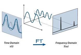
Time Domain to Frequency Domain Conversion using FFT.
source : mriquestions.com
The traveling signal is in time domain. Time domain signal comprises of multiple frequency components as shown in the image above. In order to separate out all frequency components the FFT technique is used.
For the purpose of this course we don’t have to get into mathematical details of FFT. But, it is important to understand the use of FFT in radar’s digital signal processing. It gives the frequency response of the return signal with each peak in frequency spectrum representing the detected target’s chararcterstics.
Learn more on FFT implementation here .
FFT and FMCW
L2 Output Range FFT Connected To FFT Concept From Day 1
Fast Fourier Transform
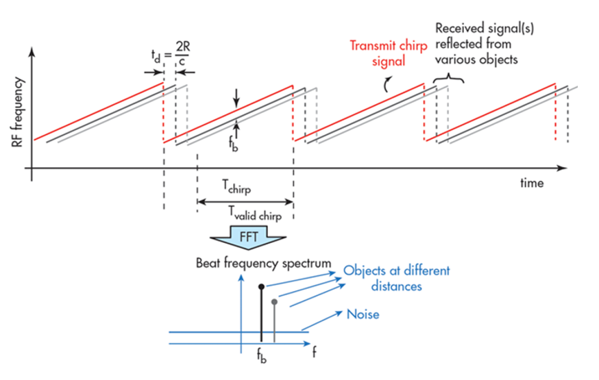
source : Texas Instruments
Range FFTs
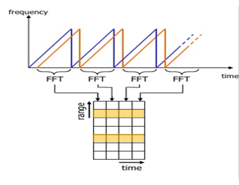
As seen in the image below, the Range FFTs are run for every sample on each chirp. Since each chirp is sampled N times, it will generate a range FFT block of N * (Number of chirps). These FFT blocks are also called FFT bins.
Range FFT
source : Delft University of Technology
Each chirp is sampled N times, and for each sample it produces a range bin. The process is repeated for every single chirp. Hence creating a FFT block of N*(Number of chirps).
Each bin in every column of block represents increasing range value, so that the end of last bin represents the maximum range of a radar.
Graphic
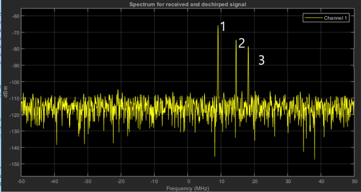
Output of Range FFT in MATLAB.
X-axis = Beat Frequency,
Y-axis = Signal power in dBm
Output of Range FFT
Above is the output of the 1st stage FFT (i.e Range FFT). The three peaks in the frequency domain corresponds to the beat frequencies of three different cars located at 150, 240 and 300 m range from the ego vehicle.
Fast Fourier Transform Exercise
Steps to Implement Range FFT
In the following exercise, you will use a Fourier transform to find the frequency components of a signal buried in noise. Specify the parameters of a signal with a sampling frequency of 1 kHz and a signal duration of 1.5 seconds.
To implement the 1st stage FFT, you can use the following steps:
- Define a signal. In this case (amplitude = A, frequency = f)
signal = A*cos(2*pi*f*t)- Run the fft for the signal using MATLAB fft function for dimension of samples N.
signal_fft = fft(signal,N);- The output of FFT processing of a signal is a complex number (a+jb). Since, we just care about the magnitude we take the absolute value (sqrt(a^2+b^2)) of the complex number.
signal_fft = abs(signal_fft);- FFT output generates a mirror image of the signal. But we are only interested in the positive half of signal length L, since it is the replica of negative half and has all the information we need.
signal_fft = signal_fft(1:L/2-1) - Plot this output against frequency.
You can use the following MATLAB starter code:
Fs = 1000;            % Sampling frequency
T = 1/Fs;             % Sampling period
L = 1500;             % Length of signal
t = (0:L-1)*T;        % Time vector

% TODO: Form a signal containing a 77 Hz sinusoid of amplitude 0.7 and a 43Hz sinusoid of amplitude 2.
S = ?

% Corrupt the signal with noise
X = S + 2*randn(size(t));

% Plot the noisy signal in the time domain. It is difficult to identify the frequency components by looking at the signal X(t).
plot(1000*t(1:50) ,X(1:50))
title('Signal Corrupted with Zero-Mean Random Noise')
xlabel('t (milliseconds)')
ylabel('X(t)')

% TODO : Compute the Fourier transform of the signal.

% TODO : Compute the two-sided spectrum P2. Then compute the single-sided spectrum P1 based on P2 and the even-valued signal length L.


% Plotting
f = Fs*(0:(L/2))/L;
plot(f,P1)
title('Single-Sided Amplitude Spectrum of X(t)')
xlabel('f (Hz)')
ylabel('|P1(f)|')
Solution
L2 Workspace
Doppler Estimation Further Research
For additional resources related to FFT, see these lecture notes .